Gilts & liability hedging · September 2026
The gilt hedging journey
How do you turn a pension payment schedule into a portfolio of government bonds?
Build the pension promise, see what each gilt contributes, then assemble the hedge. The remaining gaps tell us when cash must be invested or borrowed—and where changes in rates still matter.
01 / The liability
Build the pension promise
Start with 400 pensioners aged 55–65. Each receives £36,000 a year for the rest of their life. Weight each future payment by the chance that it will be made, then discount it back to today.
A payment due in ten years depends on interest rates over all ten years. Its rate exposure is a box extending from today to the payment date. Add the boxes for every payment and every member, and the liability takes shape.
Loading the chart…
Read the shape. Near-term rates affect almost every payment, so exposure is highest on the left. Further along, only the later payments remain. A rise in rates reduces present value; the chart shows the magnitude of that sensitivity.
The area under the curve is the approximate value change for a one basis point parallel move in forward rates. One basis point is 0.01 percentage points.
Liability assumptions
The 400 ages are equally spaced from 55 to 65. Payments are £36,000 annually in arrears, conditional on survival, for years 1–60. The Gompertz mortality hazard is 1% at age 60 and increases by a factor of e every nine years. All cashflows use a flat 4% continuously compounded discount curve. The paper gives the survival formula and the complete inputs.
02 / The instruments
See what each gilt can contribute
A gilt makes coupon payments and repays its principal at maturity. Those payments create another staircase of rate exposure. The task is to combine the available staircases into something close to the liability.
Compare any of the 61 gilts in the specified universe. Here, each gilt is scaled to the same starting height as the liability so that its shape is easy to see.
Loading the chart…
Read the steps. A small drop marks a coupon payment. The large final drop is the principal repayment. Shorter gilts stop contributing earlier; longer gilts carry exposure further along the curve.
Move over a curve to inspect it, or drag across a region to zoom. The next stage uses the actual amounts held in the hedge.
03 / The portfolio
Assemble the hedge
The exposure transport calculation selects 46 gilts and sizes each position. Play the build-up to add them from longest to shortest maturity and watch the hedge approach the liability.
The animation follows the holdings in the completed solution. Switch to the residual view to see where the resulting portfolio holds too much or too little exposure.
Loading the chart…
Latest addition: 3.75% 2027 · £2,537,587 nominal
Read the fit. The final hedge leaves 2.6% of the liability’s exposure unmatched, measured by the absolute gap between the curves. The resulting 97.4% fit summarises the shape.
Exposure transport chooses weights by minimising cumulative mismatch along the maturity axis. The method below explains that objective and how it differs from the displayed fit measure.
The completed hedge
Same initial investment. Different payment dates.
The hedge costs the same as the liability’s present value. It also has the same total sensitivity to a parallel change in forward rates. These two constraints leave the optimiser to choose how the exposure—and the cash needed between payments—is distributed through time.
| Measure | Liability | Gilt hedge |
|---|---|---|
| Present value | £173,640,556 | £173,640,556 |
| Parallel PV01 | £166,310 / bp | £166,310 / bp |
The £4,292 per bp absolute residual adds the gaps across all maturities without allowing positive and negative gaps to cancel. For a parallel move those signed gaps cancel; for a change in the shape of the curve they may not.
Between payments, the portfolio reaches £5.82m of discounted financing need. Adding a £3m ceiling raises the transport objective by 47.6%. The financing example shows how this limit changes the portfolio.
Inspect the 46 holdings
| Line | Gilt | Maturity | Nominal amount | Market value |
|---|---|---|---|---|
| 1 | 1.125% 2073 | 47.62y | £101 | £39 |
| 2 | 1.625% 2071 | 45.61y | £838 | £423 |
| 3 | 3.5% 2068 | 42.37y | £24,669 | £22,092 |
| 4 | 2.5% 2065 | 39.36y | £91,270 | £63,989 |
| 5 | 4% 2063 | 37.61y | £203,853 | £205,414 |
| 6 | 0.5% 2061 | 35.62y | £419,535 | £141,158 |
| 7 | 4% 2060 | 33.86y | £1,084,197 | £1,082,005 |
| 8 | 1.75% 2057 | 31.36y | £2,039,229 | £1,217,730 |
| 9 | 4.25% 2055 | 29.74y | £2,049,228 | £2,145,795 |
| 10 | 4.375% 2054 | 28.39y | £2,202,942 | £2,337,496 |
| 11 | 1.5% 2053 | 27.39y | £2,062,363 | £1,202,690 |
| 12 | 3.75% 2052 | 26.36y | £2,935,426 | £2,812,853 |
| 13 | 1.25% 2051 | 25.39y | £2,482,335 | £1,392,471 |
| 14 | 0.625% 2050 | 24.62y | £3,320,910 | £1,570,251 |
| 15 | 4.25% 2049 | 23.74y | £2,429,504 | £2,533,541 |
| 16 | 1.75% 2049 | 22.87y | £6,035,240 | £3,998,894 |
| 17 | 1.5% 2047 | 21.36y | £6,786,779 | £4,349,281 |
| 18 | 4.25% 2046 | 20.74y | £2,098,186 | £2,182,691 |
| 19 | 0.875% 2046 | 19.89y | £6,392,089 | £3,650,450 |
| 20 | 3.5% 2045 | 18.87y | £6,166,017 | £5,757,635 |
| 21 | 3.25% 2044 | 17.86y | £7,251,154 | £6,558,636 |
| 22 | 4.5% 2042 | 16.74y | £8,305,147 | £8,862,742 |
| 23 | 1.25% 2041 | 15.61y | £7,736,593 | £5,291,993 |
| 24 | 4.25% 2040 | 14.74y | £5,910,303 | £6,111,895 |
| 25 | 4.375% 2040 | 13.89y | £7,543,717 | £7,846,378 |
| 26 | 4.25% 2039 | 13.49y | £44,642 | £45,628 |
| 27 | 1.125% 2039 | 12.89y | £8,220,337 | £5,840,971 |
| 28 | 3.75% 2038 | 11.89y | £3,007,285 | £2,938,447 |
| 29 | 1.75% 2037 | 11.49y | £11,543,195 | £9,134,009 |
| 30 | 4.25% 2036 | 9.99y | £10,811,092 | £11,001,304 |
| 31 | 0.625% 2035 | 9.39y | £4,073,607 | £2,998,689 |
| 32 | 4.5% 2034 | 8.49y | £7,026,812 | £7,260,211 |
| 33 | 4.625% 2034 | 7.89y | £6,450,012 | £6,735,161 |
| 34 | 0.875% 2033 | 7.39y | £1,154,195 | £923,911 |
| 35 | 3.25% 2033 | 6.89y | £7,636,259 | £7,303,311 |
| 36 | 4.25% 2032 | 6.24y | £1,549,786 | £1,584,619 |
| 37 | 1% 2032 | 5.89y | £6,970,484 | £5,876,101 |
| 38 | 0.25% 2031 | 5.39y | £3,773,877 | £3,088,849 |
| 39 | 4.75% 2030 | 4.74y | £5,042,421 | £5,256,605 |
| 40 | 4.375% 2030 | 3.99y | £9,463,488 | £9,584,503 |
| 41 | 4.125% 2029 | 3.36y | £852,755 | £859,726 |
| 42 | 0.5% 2029 | 2.89y | £7,529,286 | £6,812,843 |
| 43 | 4.375% 2028 | 1.99y | £8,186,957 | £8,243,134 |
| 44 | 0.125% 2028 | 1.89y | £981,061 | £912,003 |
| 45 | 1.25% 2027 | 1.36y | £3,492,099 | £3,370,374 |
| 46 | 3.75% 2027 | 0.99y | £2,537,587 | £2,531,614 |
| Total of displayed positions | £195,918,861 | £173,640,556 | ||
Nominal amount is the face value held; market value is its cost at the valuation date. Individual positions are rounded to whole pounds. The optimiser chooses continuous position sizes. The CSV retains the unrounded amounts.
The research question
How far away is the offset?
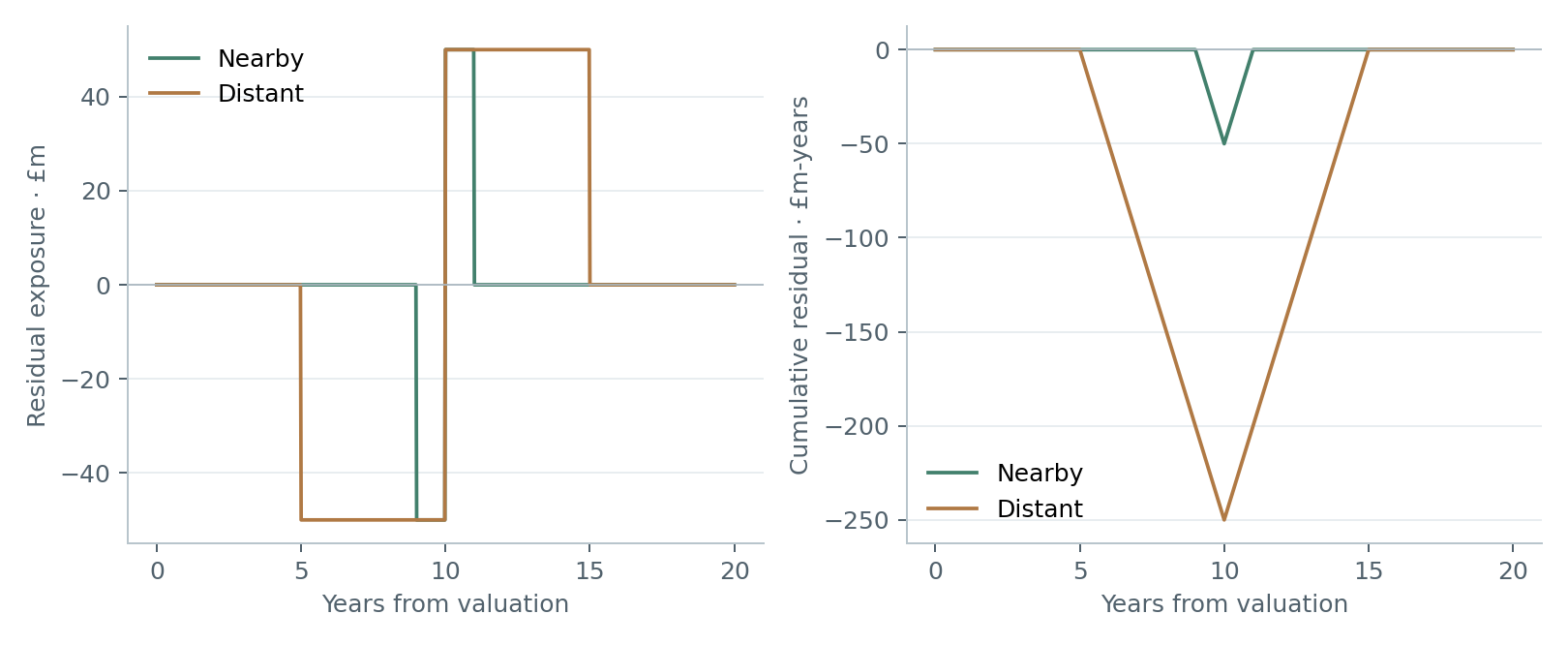
Suppose a pension payment is due in year ten. You could support it with bonds paying in years nine and eleven, or in years five and fifteen. Both combinations can match its present value and total rate sensitivity. The second relies on rates staying aligned across a much longer stretch of the curve.
What transport measures
Accumulate the difference between hedge and liability exposure. The area under the absolute value of that accumulated balance measures how much exposure needs an offset, and how far away that offset is.
Minimise ∫ |H(u)| du
The calculation holds initial investment and total PV01 equal. It selects long-only positions with the smallest worst first-order loss when the maturity slope of rate shocks is bounded.
What the fit percentage measures
The displayed fit measures the absolute gap between the two exposure curves, relative to total liability exposure. It is a simple way to read the chart.
Close offsets can reduce exposure to relative-rate changes while still requiring substantial cash between payments. The paper adds a financing limit directly to the portfolio calculation.
Four objectives · one common budget
The rate model changes the preferred hedge
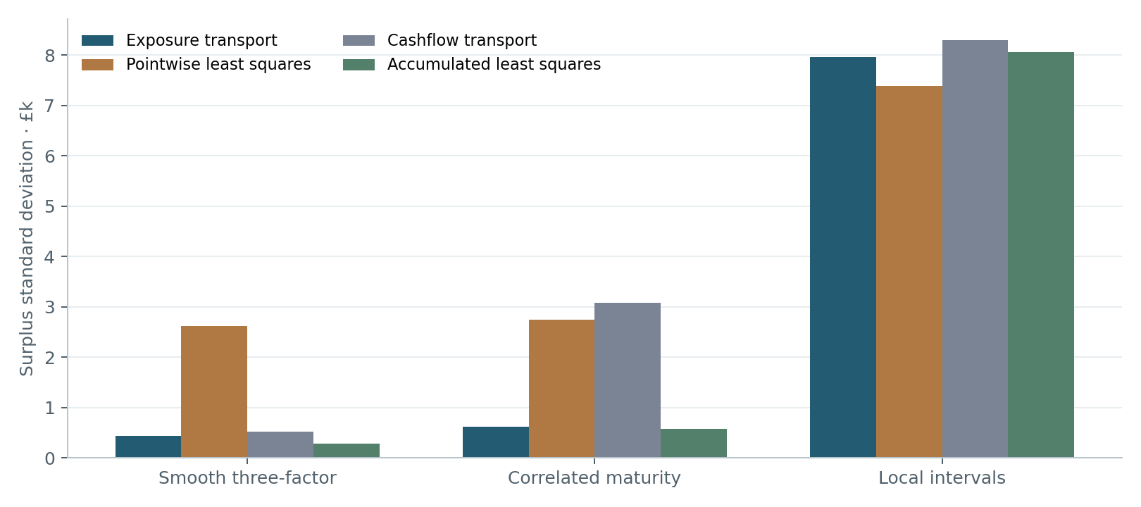
The paper compares exposure transport, cashflow transport and two forms of least squares on the same pension payments and gilt universe. Each portfolio faces the same 15,000 curve shocks.
Accumulated least squares gives the lowest dispersion in the smooth and correlated scenarios. Pointwise least squares leads under independent local shocks. Exposure transport minimises the separate worst-case criterion defined by a bound on maturity slopes.
Read the research
Hedging liabilities from their cashflows
The financing identity, the transport result, examples you can check by hand, and a fully specified pension and gilt experiment.
Read the working paperCalculation and data
The example uses an explicitly specified flat discount curve, survival formula and set of 61 gilt payment schedules. Every price and position is calculated from those inputs. The portfolio matches both present value and PV01, with continuous long-only holdings.
The transport objective is integrated exactly between payment dates, including intervals where the accumulated residual crosses zero. The replication package checks the cashflow identities, analytic examples, budget constraints, scenario summaries and a numerical bound on the optimum.
Model assumptions · Payment schedules · Interactive chart data